---
title: "N-grams and Word Sequences"
engine: knitr
format:
html:
fig-width: 10
fig-height: 12
dpi: 300
editor_options:
chunk_output_type: inline
---
```{r}
#| include: false
# This is just to render the document correctly in the CI/CD pipeline
library(tidyverse)
library(tidytext)
comments <- readr::read_csv("../../data/clean/comments_preprocessed.csv")
```
As you can notice, counting words can be useful to explore common terms in a text corpus, but it does not capture the context in which words are used. To gain deeper insights into the relationships between words, we can analyze sequences of words, known as **n-grams**. N-grams are contiguous sequences of 'n' items (words) from a given text. For example, a bigram is a sequence of two words, while a trigram is a sequence of three words.
## Creating N-grams
Because creating n-grams involves tokenizing text into sequences of words, we can use the `unnest_tokens()` function from the `tidytext` package again, but this time specifying the `token` argument to create n-grams.
```{r}
# Creating bigrams (2-grams) from the comments
ngrams <- comments %>%
  unnest_tokens(ngrams, comments, token = "ngrams", n = 2) #bigrams

ngrams
```
The resulting `ngrams` data frame contains bigrams extracted from the comments. Each row represents a bigram, which consists of two consecutive words from the original text.
By changing the value of `n` in the `unnest_tokens()` function, we can create trigrams (3-grams), four-grams, and so on, depending on our analysis needs.
```{r}
# Creating trigrams (3-grams) from the comments
trigrams <- comments %>%
  unnest_tokens(ngrams, comments, token = "ngrams", n = 3) #trigrams
trigrams
```
## Next Word Prediction Using N-grams
One practical application of n-grams is in building simple predictive text models. For instance, we can create a function that predicts the next word based on a given word using bigrams.
```{r}
# Function to predict the next word based on a given word using bigrams
next_word <- function(word, ngrams_df) {
    matches <- ngrams_df %>%
        separate(ngrams, into = c("w1", "w2"), sep = " ", remove = FALSE) %>%
        filter(w1 == word) %>%
        pull(w2)
    freq <- table(matches)
    nw <- max(freq)
    return(names(freq[freq == nw]))
}
```
This function takes a word and the n-grams data frame as inputs, finds all bigrams where the first word matches the input word, and returns the most frequently occurring second word as the predicted next word.
We can see how this function works by providing an example:
```{r}
type_any_word = "ben"

next_word(type_any_word, ngrams)
```
We can even play with a simple loop to see how the prediction evolves:
```{r}
current_word = "wow"
for (i in 1:5) {
  predicted_word = next_word(current_word, ngrams)
  cat(current_word, "->", predicted_word, "\n")
  current_word = predicted_word
}
```
If you have played with this code, you might notice that the predictions can sometimes lead to repetitive or nonsensical sequences. This is a limitation of using simple n-gram models without additional context or smoothing techniques. We can explore by using trigrams to see if predictions improve:
```{r}
# Function to predict the next word based on a given two-word phrase using trigrams
next_word_trigram <- function(phrase, trigrams_df) {
    words <- unlist(strsplit(phrase, " "))
    if (length(words) != 2) {
        stop("Please provide a two-word phrase.")
    }
    matches <- trigrams_df %>%
        separate(ngrams, into = c("w1", "w2", "w3"), sep = " ", remove = FALSE) %>%
        filter(w1 == words[1], w2 == words[2]) %>%
        pull(w3)
    freq <- table(matches)
    nw <- max(freq)
    return(names(freq[freq == nw]))
}
```
To use this function you would provide a two-word phrase, for instance "best show":
```{r}
type_any_phrase = "best show"
next_word_trigram(type_any_phrase, trigrams)
```
## From N-grams to Collocations
While n-grams capture all consecutive word sequences, not all of them are equally meaningful. **Collocations** are word combinations that occur together more frequently than would be expected by chance. They represent meaningful multi-word expressions like "strong coffee," "make a decision," or in our data, perhaps "plot twist" or "character development."
The key difference:
- **N-grams**: mechanical extraction of all consecutive words
- **Collocations**: statistically significant word pairs that carry specific meaning
### Identifying Collocations
To find collocations, we need to measure how "associated" two words are. One common metric is **Pointwise Mutual Information (PMI)**, which compares how often words appear together versus how often we'd expect them to appear together if they were independent.
::: {.callout-note title="Other Collocation Metrics" collapse="true"}
While we use PMI in this workshop, there are several other statistical measures commonly used to identify collocations:
- **Chi-square (χ²)**: Tests the independence of two words by comparing observed vs. expected frequencies. Higher values indicate stronger association.
- **Log-likelihood ratio (G²)**: Similar to chi-square but more reliable for small sample sizes. Commonly used in corpus linguistics.
- **T-score**: Measures the confidence in the association between two words. Less sensitive to low-frequency pairs than PMI.
- **Dice coefficient**: Measures the overlap between two words' contexts. Values range from 0 to 1.
Each metric has different strengths. PMI favors rare but strongly associated pairs, while t-score is more conservative and favors frequent collocations. The choice depends on your research goals and corpus characteristics.
:::
First, let's separate our bigrams and count them:
```{r}
library(tidyr)

# Separate bigrams into individual words and count
bigram_counts <- ngrams %>%
  separate(ngrams, into = c("word1", "word2"), sep = " ", remove = FALSE) %>%
  count(word1, word2, sort = TRUE)

head(bigram_counts, 10)
```
Now we'll calculate PMI for each bigram. PMI is calculated as:
$$\text{PMI}(w_1, w_2) = \log_2\left(\frac{P(w_1, w_2)}{P(w_1) \times P(w_2)}\right)$$
Where:
- $P(w_1, w_2)$ is the probability of the bigram occurring
- $P(w_1)$ and $P(w_2)$ are the probabilities of each word occurring independently
```{r}
library(dplyr)

# Calculate individual word frequencies
word_freqs <- comments %>%
  unnest_tokens(word, comments) %>%
  count(word, name = "word_count")

# Total number of words in corpus
total_words <- sum(word_freqs$word_count)

# Total number of bigrams
total_bigrams <- sum(bigram_counts$n)

# Calculate PMI
collocations <- bigram_counts %>%
  left_join(word_freqs, by = c("word1" = "word")) %>%
  rename(word1_count = word_count) %>%
  left_join(word_freqs, by = c("word2" = "word")) %>%
  rename(word2_count = word_count) %>%
  mutate(
    # Probability of bigram
    p_bigram = n / total_bigrams,
    # Probability of each word
    p_word1 = word1_count / total_words,
    p_word2 = word2_count / total_words,
    # PMI calculation
    pmi = log2(p_bigram / (p_word1 * p_word2))
  ) %>%
  arrange(desc(pmi))

head(collocations, 15)
```
High PMI values indicate strong collocations, that means word pairs that appear together much more than chance would predict.
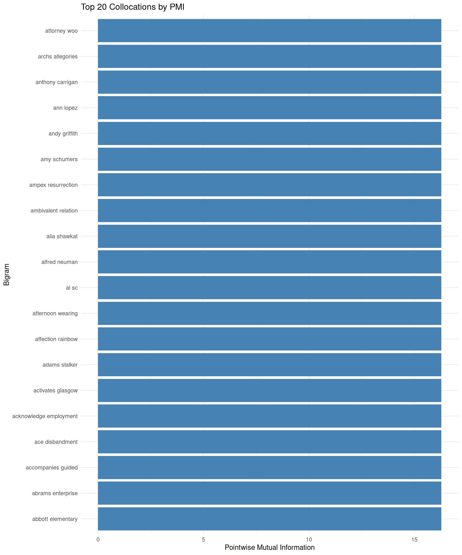
### Visualizing Collocations
Let's visualize the strongest collocations to see what meaningful phrases emerge from our Severance comments:
```{r}
library(ggplot2)

# Top 20 collocations by PMI
top_collocations <- collocations %>%
  head(20) %>%
  unite(bigram, word1, word2, sep = " ")

ggplot(top_collocations, aes(x = reorder(bigram, pmi), y = pmi)) +
  geom_col(fill = "steelblue") +
  coord_flip() +
  labs(
    title = "Top 20 Collocations by PMI",
    x = "Bigram",
    y = "Pointwise Mutual Information"
  ) +
  theme_minimal()
```
### Using Collocations for Smarter Prediction
Remember our simple n-gram predictor that sometimes got stuck in loops? We can create a more "intelligent" predictor using collocations instead of raw frequency counts. The idea is simple: instead of picking the most frequent next word, we pick the word with the highest PMI (strongest association).
```{r}
# Function to predict next word using collocation strength (PMI)
next_word_collocation <- function(word, collocations_df, min_freq = 2) {
    candidates <- collocations_df %>%
        filter(word1 == word, n >= min_freq, pmi > 0) %>%
        arrange(desc(pmi))

    # Return the word with highest PMI, or NA if no matches
    if (nrow(candidates) > 0) {
        return(candidates$word2[1])
    } else {
        return(NA)
    }
}
```
Let's compare the two approaches side by side:
```{r}
# Compare frequency-based vs. collocation-based prediction
test_word <- "mark"

freq_prediction <- next_word(test_word, ngrams)
colloc_prediction <- next_word_collocation(test_word, collocations)

cat("Frequency-based predictor:", test_word, "->", freq_prediction, "\n")
cat("Collocation-based predictor:", test_word, "->", colloc_prediction, "\n")
```
Now let's run both predictors in a loop and see which produces more meaningful sequences:
```{r}
# Frequency-based prediction
current_word <- "wow"
for (i in 1:10) {
  predicted_word <- next_word(current_word, ngrams)
  cat(current_word, "->", predicted_word, "\n")
  current_word <- predicted_word
}
current_word <- "wow"
for (i in 1:10) {
  predicted_word <- next_word_collocation(current_word, collocations)
  if (is.na(predicted_word)) {
    cat(current_word, "-> (no strong collocation found)\n")
    break
  }
  cat(current_word, "->", predicted_word, "\n")
  current_word <- predicted_word
}
```
As you can notice, both approaches are similar in structure, both are looking for the next word based on the current word. However, the collocation-based predictor leverages statistical associations between words, potentially leading to more contextually relevant predictions. This is an example of how different text analysis techniques can produce varying results based on the underlying data and methods used.