All right, enough setup! Now we can start making requests and exploring the data.
NoteWorking with APIs is an iterative process
What we’re showing here is the result of several rounds of testing and refining. Don’t feel discouraged if your first experiments don’t work as expected—it’s normal to encounter errors and surprising results when working with APIs. The important thing is to keep experimenting, learning from the errors, and refining your approach.
The shape of data
The first thing we want to do is get a sense of the shape of the data we’re getting from the API. One interesting question is: how are items distributed across time? There are multiple ways to explore this, but perhaps the most straightforward is to use facets to get the distribution of items by year.
Additionally, we’ll filter the results to only include titles, descriptions, and dates. This makes the data easier to work with and reduces the amount we need to process.
# Defining the fields, facets, and filters outside the function call for better readabilityfields = ["sourceResource.title","sourceResource.description","sourceResource.date.begin","sourceResource.date.end"]dotted_fields = {"sourceResource.subject.name": "artificial intelligence"}try: ai_search = search_items("artificial AND intelligence", # search query fields=_join_list(fields, sep=","), # fields to include in the response facets="sourceResource.date.begin", # facets to include in the response**dotted_fields, # additional parameters (e.g. filters), page_size=5, # items per page sort_by="sourceResource.date.begin", # sort by date sort_order="asc", # oldest to newest page=1, # page number to retrieve verbose=True# print the request URL for debugging purposes )except httpx.HTTPStatusError as e:print(f"HTTP error occurred: {e}. Using preloaded data instead.") r = httpx.get(f"{FALLBACK_DATA_URL}dpla_search_results.json") r.raise_for_status() ai_search = r.json()# download the preloaded data for the next stepsprint(f"{ai_search.get('count')} results found.") ifisinstance(ai_search, dict) elseprint(f"{len(ai_search)} results found.")
If the request was successful, you should see a redacted version of the request URL and the number of results found. If there was an error (e.g. invalid API key, network error, etc.), you should see an error message and the preloaded data will be used instead.
Note how the result count is significantly higher than the result from the web interface. The exact reason isn’t fully documented, but one possibility is that the web interface and API handle field matching differently (perhaps with different case sensitivity or tokenization). This is a good example of how different interfaces to the same data can yield different results, and why it’s important to understand the underlying data and how it’s indexed.
Let’s play with the facets!
Something that stands out in the response is the facet counts. Facets can be understood as a way to get aggregated counts of items based on specific fields. In this case, we’re getting the count of items by year (based on the sourceResource.date.begin field).
To explore the facet counts, we can extract the facet information from the response and plot it using a bar chart. This will let us visualize the distribution of items across time.
The first thing we need to do is reach the facet information nested in the response. To know how, we need to explore the documentation and understand the object structure.
According to the documentation, the way to reach our facet information is following this structure:
Therefore, if we want to get the entries of the sourceResource.date.begin facet, we can do it with the following code:
facets_entries = ai_search.get("facets", {}).get("sourceResource.date.begin", {}).get("entries", [])# Print a sample (we use 'time' because that's the label for date facets)for entry in facets_entries[:5]:print(f"Year: {entry.get('time')}, Count: {entry.get('count')}")
Now that we understand better the structure of the facet information, we can visualize it using a bar chart. We will use the seaborn library to create the bar chart, but you can use any other library you prefer (e.g. matplotlib, plotly, etc.).
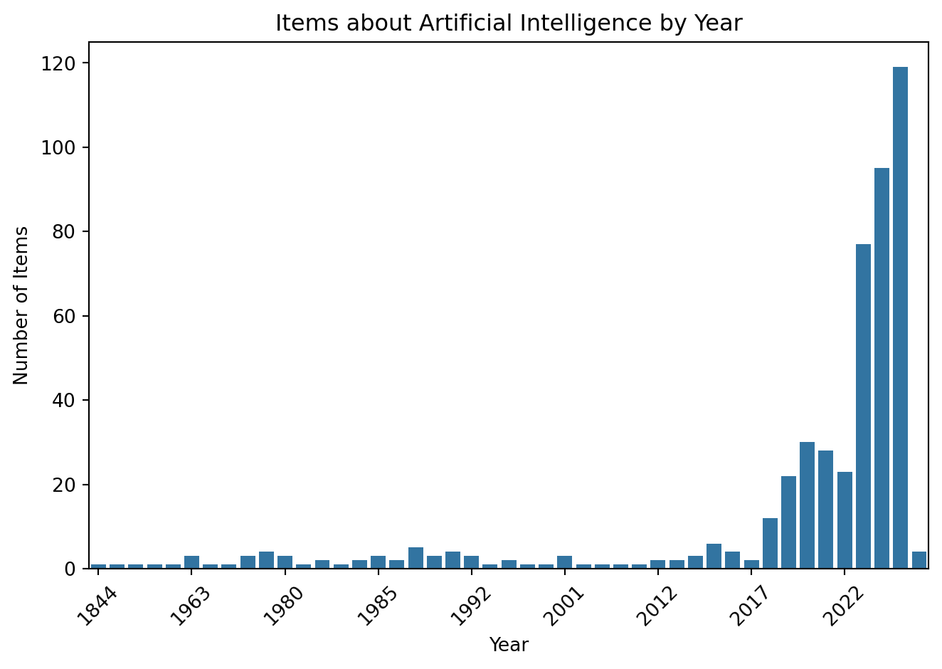
# Extract the year and count information from the facet entriesyears = [entry.get("time") for entry in facets_entries][::-1] # We use [::-1] to reverse the ordercounts = [entry.get("count") for entry in facets_entries][::-1]# Create a bar chart using seabornsns.barplot(x=years, y=counts)plt.xlabel('Year')plt.ylabel('Number of Items')plt.title('Items about Artificial Intelligence by Year')plt.xticks(range(0, len(years), 5), [years[i] for i inrange(0, len(years), 5)], rotation=45)plt.tight_layout()plt.show()
This graph helps us understand the distribution of items about artificial intelligence across different years. We can see that between 2018 and 2022 there is a peak in the number of items, and a significant increase after 2023. Before that, the number of items per year is relatively low (fewer than 10 per year).
Further exploration
With this information, we can establish three periods of interest: before 2018, between 2018 and 2022, and after 2023. We’ll set up a list with these periods and use it to filter items for further analysis:
Let’s create a pool of items for each period using the search_all_items function we defined earlier. We’ll use the sourceResource.date.begin field to filter the items by year:
ai_results = {}fields = ["sourceResource.title","sourceResource.description","sourceResource.date.begin","sourceResource.date.end"]dotted_fields = {"sourceResource.subject.name": "artificial intelligence",}try:for period_name, start_date, end_date in tqdm(periods): ai_results[period_name] = search_all_items("artificial AND intelligence", # search query max_items=400, # maximum number of items to retrieve for each period fields=_join_list(fields, sep=","), # fields to include in the response facets="sourceResource.date.begin", # Retrieve facets for date ranges page_size=100, # items per page**dotted_fields, # filter to ensure results are about AI, not just using AI in metadata**{"sourceResource.date.after": str(start_date)}, # Between year**{"sourceResource.date.before": str(end_date)}, # and Year sort_by="sourceResource.date.begin", # sort by date sort_order="asc", # oldest to newest verbose=False )except httpx.HTTPStatusError as e:print(f"HTTP error occurred: {e}. Using preloaded data instead.") r = httpx.get(f"{FALLBACK_DATA_URL}ai_results_by_wave.json") r.raise_for_status() ai_results = r.json()
This code will create a dictionary called ai_results where the keys are the period names (e.g. “preCovid”, “Covid”, “postCovid”) and the values are lists of items that match the search query and date filters for each period. Let’s print a summary of the results to see how many items we got for each period:
ai_results_summary = {period: len(items) for period, items in ai_results.items()}print("AI Results Summary by Period:")for period, count in ai_results_summary.items():print(f"{period}: {count} items")
AI Results Summary by Period:
preCovid: 89 items
Covid: 80 items
postCovid: 318 items
We can see a significant increase in the number of items in the “postCovid” period compared to the earlier periods. This reflects the AI boom that has been happening in recent years—which was likely accelerated (though not solely caused) by the COVID-19 pandemic.
Extracting keywords with YAKE
Our last step is to extract keywords from the titles and descriptions of items in each period using the YAKE library. YAKE (Yet Another Keyword Extractor) is a simple and effective unsupervised keyword extraction method.
But first, let’s explore the structure of the sourceResource field in our items:
# Get a sample item to explore the structure of the sourceResource fieldai_results.get("postCovid")[:5]
[{'sourceResource.date.begin': '2022',
  'sourceResource.date.end': '2022',
  'sourceResource.description': ['In scope of the U.S. Government Publishing Office Cataloging and Indexing Program (C&I) and Federal Depository Library Program (FDLP).',
   'Description based on online resource; title from publication (Agency website, viewed September 14, 2022).'],
  'sourceResource.title': 'Artificial intelligence strategic plan: fiscal years 2023-2027, draft report for comment'},
 {'sourceResource.date.begin': '2022',
  'sourceResource.date.end': '2022',
  'sourceResource.description': ['"Published Fall 2022."',
   '"Ann Caracristi Institute for Intelligence Research"--Cover.',
   'In scope of the U.S. Government Publishing Office Cataloging and Indexing Program (C&I) and Federal Depository Library Program (FDLP).',
   'Includes bibliographical references (pages 69-72).',
   'Description based on online resource; title from PDF title page (NIU, viewed July 18, 2023).'],
  'sourceResource.title': 'Perceptions of artificial intelligence / machine learning in the intelligence community : a systematic review of the literature'},
 {'sourceResource.date.begin': '2022',
  'sourceResource.date.end': '2022',
  'sourceResource.description': ['In scope of the U.S. Government Publishing Office Cataloging and Indexing Program (C&I) and Federal Depository Library Program (FDLP).',
   '"FHWA-HRT-21-081."',
   'Description based on online resource; title from publication (Agency website, viewed December 22, 2023).'],
  'sourceResource.title': 'Effectiveness of TMC AI applications in case studies'},
 {'sourceResource.date.begin': '2022',
  'sourceResource.date.end': '2022',
  'sourceResource.description': ['Access ID (govinfo): CHRG-117hhrg46195.',
   '"Serial no. 117-52."',
   'Includes bibliographical references.',
   'Hearing witnesses: Broussard, Meredith, Associate Professor, Arthur L. Carter Journalism Institute of New York University; Cooper, Aaron, Vice President, Global Policy, BSA--The Software Alliance; King, Meg, Director, Science and Technology Innovation Program, The Wilson Center; Vogel, Miriam, President and CEO, EqualAI; Yong, Jeffery, Principal Advisor, Financial Stability Institute, Bank for International Settlements.',
   'Date of hearing: 2021-10-13.',
   'Description based on online resource; title from PDF title page (govinfo, viewed Jan. 19, 2022).'],
  'sourceResource.title': 'Beyond I, robot : ethics, artificial intelligence, and the digital age : viritual hearing before the Task Force on Artificial Intelligence of the Committee on Financial Services, U.S. House of Representatives, One Hundred Seventeenth Congress, first session, October 13, 2021'},
 {'sourceResource.date.begin': '2022',
  'sourceResource.date.end': '2022',
  'sourceResource.description': ['Access ID (govinfo): CHRG-117hhrg47880.',
   'Hearing witnesses: Greenfield, Kevin, Deputy Comptroller for Operational Risk Policy, Office of the Comptroller of the Currency (OCC); Hall, Melanie, Commissioner, Division of Banking and Financial Institutions, State of Montana; and Chair, Board of Directors, Conference of State Bank Supervisors (CSBS); Lay, Kelly J., Director, Office of Examination and Insurance, National Credit Union Administration (NCUA); Rusu, Jessica, Chief Data, Information and Intelligence Officer, Financial Conduct Authority (FCA), United Kingdom.',
   'Date of hearing: 2022-05-13.',
   'Includes bibliographical references.',
   '"Serial no. 117-85."',
   'Description based on online resource; title from PDF title page (GovInfo, viewed Aug. 2, 2022).'],
  'sourceResource.title': 'Keeping up with the codes : using AI for effective RegTech : hybrid hearing before the Task Force on Artificial Intelligence of the Committee on Financial Services, U.S. House of Representatives, One Hundred Seventeenth Congress, second session, May 13, 2022'}]
Great! Each item is a dictionary with the following keys:
sourceResource.date.begin (str): The start date of the item (e.g. “2015-01-01”)
sourceResource.date.end (str): The end date of the item (e.g. “2015-12-31”)
sourceResource.description (str | list): A description of the item
sourceResource.title (str | list): The title of the item
Now we can use YAKE to extract keywords from the titles of the items in each period. We’ll create a function that takes a list of items and returns a dictionary with keyword counts for each period:
def extract_keywords(items, skip=None, ngram=2, max_keywords=5, language="en"):"""Extract keywords from a list of items using YAKE.""" ai_keywords = {} kw_extractor = yake.KeywordExtractor(lan=language, n=ngram, top=max_keywords)if skip: skip_keywords =set(skip)for period, items in tqdm(items.items(), desc="Extracting keywords"): period_keywords = {}for item in items: text = _join_list(item.get("sourceResource.title", "")).lower() keywords = kw_extractor.extract_keywords(text)for kw, score in keywords:if skip and kw in skip_keywords:continue period_keywords[kw] = period_keywords.get(kw, 0) +1 ai_keywords[period] = period_keywordsreturn ai_keywords
Now, we can iterate over the loaded items and extract the keywords for each period:
# Define a list of common words to skip (optional)skip_words = ["artificial intelligence", "ai", "intelligence", "artificial", "bibliographical references", "includes bibliographical", "online resource", "bibliography", "references", "bibliographical", "reference"]top =10ai_keywords = extract_keywords(ai_results, skip=skip_words, ngram=2, max_keywords=top)for period, keywords in ai_keywords.items(): sorted_keywords =sorted(keywords.items(), key=lambda x: x[1], reverse=True)[:top]print(f"Top {top} keywords for {period}:")for kw, count in sorted_keywords:print(f" {kw}: {count}")print()
Top 10 keywords for preCovid:
  machine: 9
  learning: 8
  systems: 7
  system: 6
  proceedings: 6
  machine intelligence: 5
  report: 5
  robotics: 5
  space: 5
  computer: 4

Top 10 keywords for Covid:
  sixteenth congress: 14
  hundred sixteenth: 13
  learning: 9
  report: 8
  financial services: 8
  task force: 8
  national security: 6
  national: 6
  security: 5
  united states: 5

Top 10 keywords for postCovid:
  eighteenth congress: 59
  united states: 57
  hundred eighteenth: 54
  states senate: 52
  hearing: 36
  learning: 26
  machine learning: 22
  report: 19
  nineteenth congress: 19
  hundred nineteenth: 19
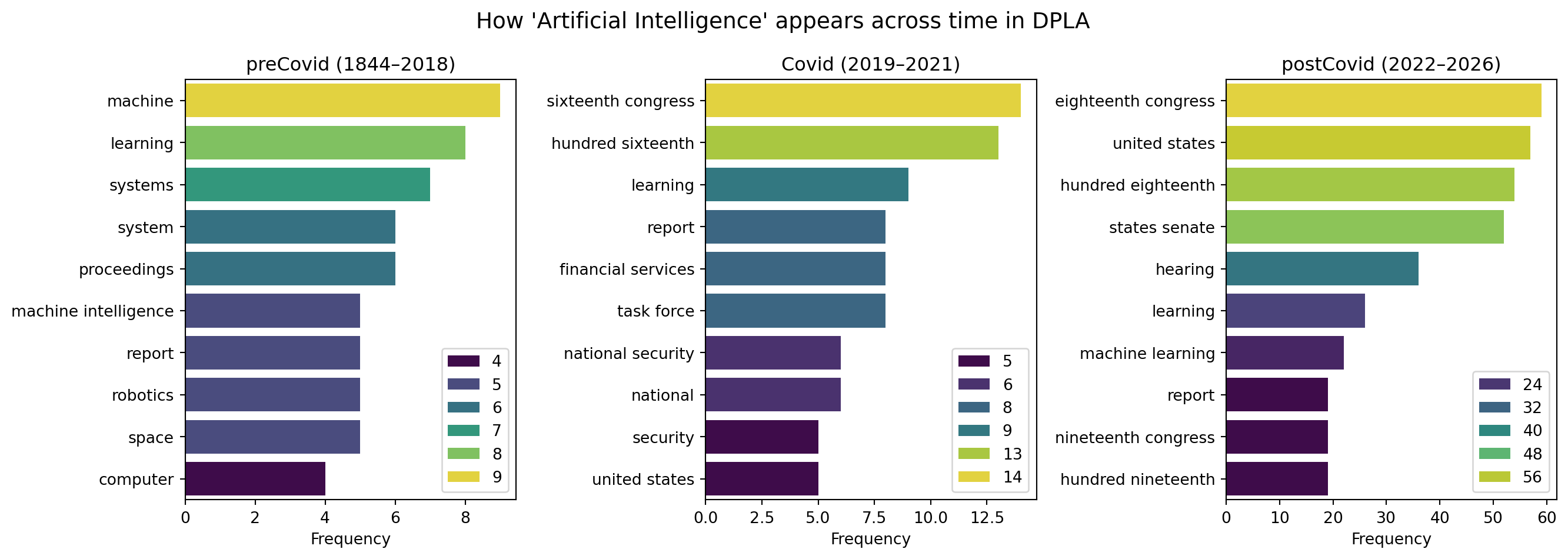
Finally, we can visualize the top keywords for each period using a bar chart:
fig, axes = plt.subplots(1, 3, figsize=(14, 5), sharex=False)for ax, (period_name, start_year, end_year) inzip(axes, periods): data = _top_n(ai_keywords.get(period_name, {}), 10) terms =list(data.keys()) counts =list(data.values()) sns.barplot(x=counts, y=terms, ax=ax, palette="viridis", hue=counts) ax.set_title(f"{period_name} ({start_year}–{end_year})") ax.set_xlabel("Frequency")plt.suptitle("How 'Artificial Intelligence' appears across time in DPLA", fontsize=14)plt.tight_layout()plt.show()
Wrapping up
And that’s it! You’ve successfully queried the DPLA API, filtered and paginated through results, visualized temporal distributions using facets, and extracted keywords from metadata across different time periods. Along the way, you’ve seen how APIs let you access much richer datasets than web interfaces alone—and how a little code can unlock powerful ways to explore and analyze cultural heritage collections.
The techniques you’ve learned here—building requests programmatically, handling pagination, working with nested JSON structures, and combining API data with text analysis—are transferable to many other APIs. Whether you’re exploring museum collections, scientific datasets, or social media archives, the same patterns apply: understand the documentation, experiment with parameters, and iterate on your queries.
Keep exploring, and remember: every API is a doorway to data that’s waiting to be discovered.